Perfect competition happens when both buyers and producers are price takers, meaning they have no (individual) influence over the price of a product.
Conditions for perfect competition:
- Large number of producers such that no individual producer's production represents a significant part of the total output in the market. Producers must sell their products (no matter the quantity) at a market price that is outside of their control (price-taker). This means that for firm that is a price-taker, its demand is perfectly elastic (horizontal).
- Producers sell homogeneous goods, meaning that consumers do not care from which sellers they buy the goods from.
- Producers do not face barriers to entry or exit. Producers are able to enter or exit the market freely.
Understanding economic graphs under perfect competition:
- The price (Pm) is determined in the market becomes the demand curve for an individual firm (remember the firm is price-taker). Then, if the demand is horizontal, it follows by the product rule in calculus, the marginal revenue is constant.
- Remember, the profit maximizing output is determined by MR=MC.
- The long run equilibrium is achieved as each individual firm is earning a normal profit (see graph above). If a firm is earning a negative or positive normal profit, firms will exit (enter) the market until a normal profit is achieved at an individual firm level.
- The firm represented on the graph produces efficiently as it is producing at the lowest point on its average total cost (ATC) curve.
- An increase in price causes an increase in output. This creates a new marginal revenue equal to the new equilibrium price (Pm2) that is bigger than the original price (Pm1).
- The firm now produces where Pm2=MR2=MC. At this point, the firm is earning a positive economic profit, in the short run, as Pm2>ATC at the new quantity being produced.
- Profit is equal to the vertical distance between Pm2 and ATC times the number of goods produced by the firm at that price.
- The firm is not productively efficient, as it is not s it is producing at the lowest point on its average total cost (ATC) curve.
In the long run, the positive economic profit attracts other firms to enter the market. This new influx of firms will move the supply curve to the right, thereby increasing supply and decreasing the equilibrium price until every firm earns a normal profit.
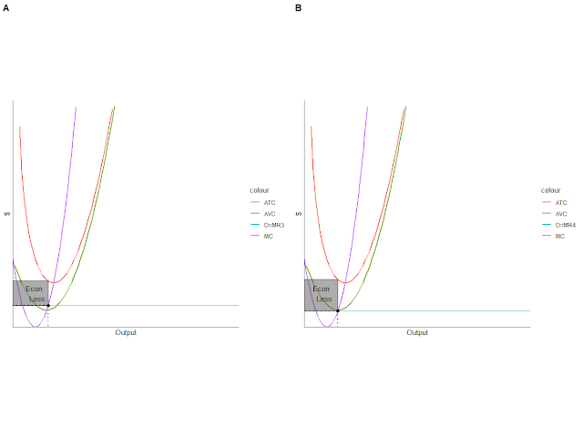
Should a firm exit the market in the short run if it faces a negative profit? It depends, if the firm is able to cover its variable costs, then it stays in the market. If it cannot cover its variable cost, the firm should exit the market immediately.
The graph on the left indicates that the firm should still operate as it is able to cover its AV costs at that price. However, the firm on the right cannot cover its ATC and has to exit the market.
In the long run, negative economic profit pushes away some firms out of the market, thereby decreasing the supply and increasing the equilibrium price, until every firm earns a normal profit.
Part A of the graph shows that due to a leftward shift in demand (from D1 to D3), the new price Pm3<Pm1. Some firms are experiencing losses and are forced out of the market, reducing supply (S1 to S3). This shift in supply happens up until every firm is making a normal profit which occurs at Pm1.
Reference: Mayer,David. AP Microeconomics Crash Course. Research & Education Association (2014). p 91-99.


Comments
Post a Comment